
There’s an informative and well-maintained Verilog section at www.asic-world.com with a tutorial.
Fun with filters
In this post, I am going to review a number of Matlab functions useful for discrete-time signal processing.
The transfer function
Suppose we have a discrete-time signal x[n] sampled with frequency Fs, and wish to pass it through a filter with output y[n]. The filter has impulse response h[n]. The output of the system y[n] is the convolution of the input and the filter, x[n]*h[n]. Taking the z-transform of the system takes convolution to multiplication, resulting in the equation
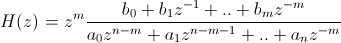
 H(z) is known as the transfer function of the filter, and is represented in the general case as a fraction B/A of two polynomials in z.
![]() In practice, it is easier to work with powers of 1/z than z, so we factor out an appropriate power of z to put H in terms of 1/z.
In practice, it is easier to work with powers of 1/z than z, so we factor out an appropriate power of z to put H in terms of 1/z.
This gives two vectors, B and A, of polynomial coefficients in ascending powers of 1/z. These vectors characterize the filter in Matlab.
A moving average filter
The basic Matlab filter command is filter.filter takes a filter [B,A] and an input vector x[n] and returns its output y[n]. Let’s create a 63-point moving average filter, with sampling frequency 1kHz. This filter “smooths” its output by averaging the last N=63 samples. This is a finite impulse response filter, so A is equal to 1. B is the average of the last 63 samples; i.e. a length 63 vector in 1/z, divided by 63.
a=1; b=ones(1,63)/63;
Now let’s look at its effect on a couple of sine waves. The output is an attenuated version of the input.
Fs=1000; t=linspace(0,2*pi,Fs); x1=sin(t);x2=sin(10*t);
y1=filter(b,a,x1);y2=filter(b,a,x2);
subplot(2,1,1); plot(t,y1); subplot(2,1,2); plot(t,y2);

Matlab z-plane functions
We can look at the entire frequency response with the freqz function. One invocation of freqz takes our filter [B,A], along with the number of (uniformly spaced) frequencies and the sampling rate Fs, and returns a plot of the frequency response from 0 to Fs. Our discrete time moving average filter is a low pass filter, with some interesting oscillating behavior compared to an analog filter (to be explored later). Note that the response is symmetric with respect to Fs/2, which is the Nyquist frequency of the input signal.
freqz(b,a,512,'whole',Fs)

The corresponding impulse response (i.e. in the time domain) is computed by the impz command. The impulse response for this uniformly weighted filter is pretty boring.
impz(b,a)

zplane produces a pole-zero plot (where the poles and zeros are the roots of the polynomials B and A, obtained from the roots command) on the complex plane.
z=roots(b);
zplane(b,a);

Monday DSP drive-by
I have found a couple of neat links for learning digital signal processing (DSP), from a practical angle. Steve Smith has a free online DSP book. If you’re into Matlab, or even you’re just using Matlab to get into DSP, you may find (another) Steve Eddins’s image processing blog less detailed, but more enlightening than help.
The color of noise
You may have heard of the term “white noise“, and seen “white noise generators” marketed as sleeping or concentration aids, without knowing exactly what white noise was. Colloquially, “white noise” may be thought of as random noise which is evenly spread over the entire frequency spectrum (Pure white noise is an idealization, but it can be approximated over a given frequency range. I won’t get into randomness here). Clearly, the term “white noise” takes its cue from “white light”, which is the sum of all colors of light before they are refracted through a prism.
In keeping with this theme, there are other “colors” of noise. There is “pink” noise, which is random noise which attenuates (or weakens) at the rate of 3 decibels per octave (i.e. it halves in power for every doubling of frequency). “Red” noise drops off at 6dB per octave. Red noise is sometimes called “Brown noise”, but Brown in this case refers to Robert Brown of Brownian motion fame, and not the color!
Going the other direction, blue noise and purple noise increase at 3dB and 6dB per octave, respectively. Each color of noise has a distinctive sound and it’s interesting to compare them. White noise generators are sometimes used to “jam” distracting ambient sounds or simply to provide relaxation. I prefer Brown noise.
Now for something useful. Linux comes with a very handy audio utility called sox which includes the ability to generate noise. I got the idea from this blog when looking for WNG software. The frontend to sox is the play command.
Here’s an example:
play -n synth brownnoise
pinknoise and whitenoise options are also available.
sox is useful for many more purposes than generating noise, so it’s definitely a utility worth looking into. For those who prefer to get their noise at retail, there’s SimplyNoise.
Icarus Verilog and freeware EDA
I recently started learning the Verilog hardware description language, and was bewildered by the size and complexity of the major commercial EDA offerings. They’re huge, expensive, Windows-based, GUI-driven monsters packed with quirks and features, aimed at teams of commercial engineers with dedicated IT staff. I’m sure they’re very useful, but they’re very imposing to somebody who just wants to compile and run Verilog testbenches. Baby steps.
One alternative is Icarus Verilog. Icarus is a tiny, free, command-line driven Verilog compiler and simulator targeted for Linux. According to the site, it’s written to Verilog 2005 (IEEE Standard 1364-2005). It’s available in recent Ubuntu, and in any event, can be easily built from source. Getting started is dead simple. Install Icarus, enter your Verilog design into text-format .v source files using your favorite editor, and compile it using the iverilog binary.
$ iverilog -o foobar foo.v bar.v
$ ./foobar
[output ...]
More examples and free EDA to follow.
Posted in Undifferentiated Goo
Tagged eda, linux, oss, verilog
Comments Off on Icarus Verilog and freeware EDA