Matlab includes classical control theory analysis functions such as for Bode plots. Bode plots are useful for determining the behavior of linear time-invariant systems in filters and controls. Again, we are working with Matlab’s tf objects. Let’s define a third-order filter, and compute the Bode plot:
>> L=tf([10000],[1 111 1110 1000]);

>> bode(L)

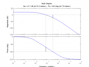
The Bode plot gives the gain (amplitude) and phase of the filter’s output compared to the input over the frequency domain. Of interest to feedback systems is the filter’s gain and phase margins and crossover frequencies. These can be determined by looking at the Bode plot, but naturally, Matlab has a function to plot them for us:
>> margin(L)
There is also a text-only command to compute these values:
>> allmargin(L)
ans =
GainMargin: 12.2210
GMFrequency: 33.3167
PhaseMargin: 54.9018
PMFrequency: 7.7980
DelayMargin: 0.1229
DMFrequency: 7.7980
Stable: 1
One definition of phase margin is the amount of phase that can be tolerated before the filter reaches 180° of phase and becomes unstable in a closed feedback loop. A minimum phase margin of 45° is typically considered for stability. From here, we can see that the filter has adequate phase margin. The phase may be related to a time delay by dividing it by the frequency. Let’s create a time-delayed copy of L, Ld, and set the time delay so that Ld is on the verge of instability.
>> Ld = L;

>> Ld.InputDelay=(54.9018*pi/180)/7.7980; allmargin(Ld)
ans =
GainMargin: [1×20 double]
GMFrequency: [1×20 double]
PhaseMargin: 1.5869e-04
PMFrequency: 7.7980
DelayMargin: 3.5518e-07
DMFrequency: 7.7980
Stable: 1
Ld’s phase margin is very near to zero, indicating a marginally stable system. Let’s nudge it over the edge.
>> Ld.InputDelay=(54.9018*pi/180)/7.7980+.0001; allmargin(Ld)

ans =
GainMargin: [1×20 double]
GMFrequency: [1×20 double]
PhaseMargin: -0.0445
PMFrequency: 7.7980
DelayMargin: -9.9645e-05
DMFrequency: 7.7980
Stable: 0
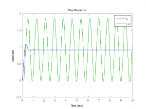
L is stable and Ld is now marginally unstable. How do we demonstrate this? One way is to plot the step response of the closed feedback loop. Note: I found Matlab needs to convert the tf objects into a state-space model with the ss() function to work with time delays. L reaches equilibrium after a brief overshoot, whereas Ld oscillates with increasing amplitude. In fact, since Ld is unstable, it will eventually shoot off to infinity, in our ideal world of functions.
hold on; step(ss(L)/(1+ss(L)),10); step(ss(Ld)/(1+ss(Ld)),10); legend('L','Ld')

