
In this post, I am going to review a number of Matlab functions useful for discrete-time signal processing.
The transfer function
Suppose we have a discrete-time signal x[n] sampled with frequency Fs, and wish to pass it through a filter with output y[n]. The filter has impulse response h[n]. The output of the system y[n] is the convolution of the input and the filter, x[n]*h[n]. Taking the z-transform of the system takes convolution to multiplication, resulting in the equation
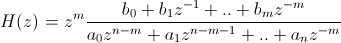
 H(z) is known as the transfer function of the filter, and is represented in the general case as a fraction B/A of two polynomials in z.
![]() In practice, it is easier to work with powers of 1/z than z, so we factor out an appropriate power of z to put H in terms of 1/z.
In practice, it is easier to work with powers of 1/z than z, so we factor out an appropriate power of z to put H in terms of 1/z.
This gives two vectors, B and A, of polynomial coefficients in ascending powers of 1/z. These vectors characterize the filter in Matlab.
A moving average filter
The basic Matlab filter command is filter.filter takes a filter [B,A] and an input vector x[n] and returns its output y[n]. Let’s create a 63-point moving average filter, with sampling frequency 1kHz. This filter “smooths” its output by averaging the last N=63 samples. This is a finite impulse response filter, so A is equal to 1. B is the average of the last 63 samples; i.e. a length 63 vector in 1/z, divided by 63.
a=1; b=ones(1,63)/63;
Now let’s look at its effect on a couple of sine waves. The output is an attenuated version of the input.
Fs=1000; t=linspace(0,2*pi,Fs); x1=sin(t);x2=sin(10*t);
y1=filter(b,a,x1);y2=filter(b,a,x2);
subplot(2,1,1); plot(t,y1); subplot(2,1,2); plot(t,y2);

Matlab z-plane functions
We can look at the entire frequency response with the freqz function. One invocation of freqz takes our filter [B,A], along with the number of (uniformly spaced) frequencies and the sampling rate Fs, and returns a plot of the frequency response from 0 to Fs. Our discrete time moving average filter is a low pass filter, with some interesting oscillating behavior compared to an analog filter (to be explored later). Note that the response is symmetric with respect to Fs/2, which is the Nyquist frequency of the input signal.
freqz(b,a,512,'whole',Fs)

The corresponding impulse response (i.e. in the time domain) is computed by the impz command. The impulse response for this uniformly weighted filter is pretty boring.
impz(b,a)

zplane produces a pole-zero plot (where the poles and zeros are the roots of the polynomials B and A, obtained from the roots command) on the complex plane.
z=roots(b);
zplane(b,a);
