I am a fan of Linear‘s LTSpice for casual circuit simulation. It is intuitive, simple, and free! Unfortunately, SPICE is not so simple, and documentation tends to be scattered and out of date. Here is a link with some poorly-documented parameters useful to LTSpice users.
VHDL type conversions
I have been learning VHDL for simulation and synthesis lately. Coming from a Verilog background, one of the biggest differences between Verilog and VHDL is the latter’s type system. VHDL is strongly typed, even compared to C or C++. Every signal has a type, and the compiler will tolerate very little ambiguity between types. It is fair to say you will get nowhere with VHDL until you are comfortable working with them.
Types
VHDL supports many types, but you can get by with a small number of them for logic synthesis, including std_logic, std_logic_vector, signed, unsigned, integer. The types are defined by IEEE 1164, implemented in the std_logic_1164 library. While we’re on the subject, you will also want to use the numeric_std and possibly std_logic_unsigned libraries for helper functions.
Example header:
library IEEE;
use IEEE.std_logic_1164.all;      -- for logic types
use IEEE.numeric_std.all;         -- for signed/unsigned arithmetic
use IEEE.std_logic_unsigned.all;  -- for std_logic_vector arithmetic
I will briefly describe the types:
std_logic is a single multi-valued logic bit. Most often, it will be driven either as ‘0’ (logic 0/false) or ‘1’ (logic 1/true). It supports 1-bit logical operations.
Example declaration and initialization:
signal s0 : std_logic := '1';
std_logic_vector, signed, unsigned are all bit vectors, or fixed size arrays of std_logic bits. They should be thought of primarily as bit vectors, and not numbers in the usual sense. A limited number of arithmetic functions are available, and the operands must be explicitly cast or converted into the same type.
Example declaration and initialization (note double quotes):
signal v1: std_logic_vector(3 downto 0) := "1011";  -- binary 1011
signal u1: unsigned(3 downto 0) := "1011";          -- decimal 11 (unsigned)
signal s1: signed(3 downto 0) := "1011";            -- decimal -5 (signed 2's complement)
std_logic_vector supports bitwise logical operations. It will also support unsigned arithmetic with the ieee.std_logic_unsigned package. signed and unsigned support arithmetic with numeric_std.
The integer is a different animal. It is a number. Unless constrained, it will be in the full range defined by the implementation (currently signed 32-bit). The integer will need to be constrained for the integer to be converted to a smaller number of wires. Integers are more intuitive to work with internally, but all interfaces should be implemented using one of the vector types (preferably std_logic_vector).
Example:
signal i1: integer range 0 to 15; -- 4 bits
Type Conversions
In general, one of the array types can be cast to another type of the same size:
u1 <= unsigned(v1);          -- unsigned cast
s1 <= signed(u1);            -- signed cast
v1 <= std_logic_vector(s1);  -- std_logic_vector cast
A conversion function (to_x) must be used to convert between integers and signed/unsigned types. Two operations, a conversion and a cast, are required to convert between integer and std_logic_vector. Note that unlike the cast, the conversion function takes a second argument, length, to constrain the integer to a fixed number of bits.
Example:
u1 <= to_unsigned(i1, 4);    -- unsigned conversion
s1 <= to_signed(i1, 4);      -- signed conversion
v1 <= std_logic_vector(u1);  -- std_logic_vector cast

i1 <= to_integer(s1);        -- integer conversion
The takeaway from this is that for logic synthesis, I find it useful to think of VHDL bottom-up as a symbolic representation of discrete logic (ports and wires) rather than top-down as a logical implementation of the high-level design.
No Disassembly Allowed
This WSJ article mentions Apple’s withdrawal from the EPEAT standard for “green” consumer electronics products, which includes ease of disassembly for the purpose of recycling components. Apparently, the tradeoffs necessary for complying with the standard conflict with Apple’s priority on design.
I obtained first-hand experience with Apple’s hostility to disassembly when attempting to replace the battery in my iPod Touch 3G (the Touch is basically the iPhone without the phone). This is a $300+ USD device; since the Li batteries only last a couple of years, I expect to be able to change the battery on my own. AppleCare charges $80 to change the battery, although there are many third-party mail-order shops that will charge somewhat less.
This is not simple price gouging. Replacing the battery on the iPod Touch is not an easy job. The ease of replacing the battery, or performing any sort of maintenance on the Touch beside wiping the screen, was not considered, if not actively conspired against. For starters, the battery leads are soldered onto the circuit board. Imagine working on a car directly hooked up to its battery, with no ignition switch…or working on the wiring of a house without breakers. To make matters worse, the battery is hidden behind the digitizer, LCD screen, and metal plate, which are held together with microscopic screws and liberal amounts of glue. The digitizer and LCD are quite fragile and susceptible to electrostatic discharge. It is quite challenging to unscrew, unglue, and disconnect the assembly without breaking one or more of the components. Lastly, the iPod assembly is pressure-fitted with a plastic gasket into a metal shell and held in with tabs. Removing the assembly from the shell requires special tools and a good deal of finesse to avoid damage. A picture being worth a thousand words, and a video being thousands of pictures, this video can make a suitable impression of the level of difficulty involved (I did manage to replace the battery, along with the LCD and digitizer, for about $25 shipped in parts, not counting my time).
I have sort of a love-hate relationship with Apple. The artist in me admires its (and let’s face it, I mean Jobs’s) vision and leadership. Few companies are able to inspire and lead their customers the way Apple does. On the other hand, the engineer in me hates its walled-garden mentality and hostility to tinkering.
Computer vision with OpenCV
I recently began working on a project that requires a computer to recognize objects from a video feed.
Computers can do many things more efficiently than humans, but currently, seeing things is not one of them. Discriminating arbitrary objects from a background and one another, identifying objects, and tracking movement, for instance, are things we animals can do without thinking, but computers still have great difficulty doing quickly, if at all. Many object recognition algorithms have been invented; but none of them are great, the good ones are not fast, and the fast ones are not good. I anticipate the field of computer vision will continue be fertile ground for Ph. D. theses for the next 20 years, at which point advances in computing power will allow brute force to overcome inefficiency. The OpenCV library provides a set of primitives and functions for computer vision, and should be the starting point for any aspiring computer vision-ary.
Unfortunately, OpenCV is very much a work-in-progress, as is computer vision. It provides C, C++, and Python bindings. The main API was recently changed from C to C++, but most existing documentation refers to the C API, which uses different functions. The online documentation is limited, and the OpenCV “user manual” is an O’Reilly book that is woefully out of date. A couple of sites I have found useful, recent OpenCV information at are AI Shack and Computer Vision Talks.
Problems vs. products (via the Segway)
Fun page about a DIY Segway here. I will remember the Segway as one of the most overhyped gadgets in an age of hype. The technology behind the Segway’s self-balancing trick was not innovative, but rather a straightforward application of control to the inverted pendulum problem. The Segway illustrates one of the differences between engineering and business. Engineers solve problems. Businesspeople create products and services to meet a demand. Be careful when mixing the two. A successful product is most commonly not a solution to a problem, but a novel application of existing solutions. In the case of the Segway, the novelty was there, but the demand proved to be mostly illusory.
Matlab Bode and Nyquist plots
Matlab includes classical control theory analysis functions such as for Bode plots. Bode plots are useful for determining the behavior of linear time-invariant systems in filters and controls. Again, we are working with Matlab’s tf objects. Let’s define a third-order filter, and compute the Bode plot:
>> L=tf([10000],[1 111 1110 1000]);

>> bode(L)
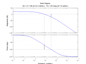
The Bode plot gives the gain (amplitude) and phase of the filter’s output compared to the input over the frequency domain. Of interest to feedback systems is the filter’s gain and phase margins and crossover frequencies. These can be determined by looking at the Bode plot, but naturally, Matlab has a function to plot them for us:
>> margin(L)
There is also a text-only command to compute these values:
>> allmargin(L)
ans =
GainMargin: 12.2210
GMFrequency: 33.3167
PhaseMargin: 54.9018
PMFrequency: 7.7980
DelayMargin: 0.1229
DMFrequency: 7.7980
Stable: 1
One definition of phase margin is the amount of phase that can be tolerated before the filter reaches 180° of phase and becomes unstable in a closed feedback loop. A minimum phase margin of 45° is typically considered for stability. From here, we can see that the filter has adequate phase margin. The phase may be related to a time delay by dividing it by the frequency. Let’s create a time-delayed copy of L, Ld, and set the time delay so that Ld is on the verge of instability.
>> Ld = L;

>> Ld.InputDelay=(54.9018*pi/180)/7.7980; allmargin(Ld)
ans =
GainMargin: [1×20 double]
GMFrequency: [1×20 double]
PhaseMargin: 1.5869e-04
PMFrequency: 7.7980
DelayMargin: 3.5518e-07
DMFrequency: 7.7980
Stable: 1
Ld’s phase margin is very near to zero, indicating a marginally stable system. Let’s nudge it over the edge.
>> Ld.InputDelay=(54.9018*pi/180)/7.7980+.0001; allmargin(Ld)

ans =
GainMargin: [1×20 double]
GMFrequency: [1×20 double]
PhaseMargin: -0.0445
PMFrequency: 7.7980
DelayMargin: -9.9645e-05
DMFrequency: 7.7980
Stable: 0
L is stable and Ld is now marginally unstable. How do we demonstrate this? One way is to plot the step response of the closed feedback loop. Note: I found Matlab needs to convert the tf objects into a state-space model with the ss() function to work with time delays. Continue reading
More Matlab filtering
Previously, I covered discrete-time filters. Matlab has functions for continuous-time filters as well. The transform of interest is the Laplace transform. As before, we obtain a transfer function, this time in the s-domain. We have the numerator B(s) and denominator A(s) in descending powers of s. It is common, but not necessary, to normalize the leading term of A to 1. Suppose
B=[5];A=[1,2,3];
Through basic algebra, we have the partial fraction expansion
Matlab can calculate the partial fraction expansion of this function with the residue command. The output vectors r,p,k contain the residues (r terms above), poles (p terms), and the direct term k, which is not present in this function.
[r,p,k]=residue(B,A);

r =
        0 - 1.7678i
        0 + 1.7678i
p =
  -1.0000 + 1.4142i
  -1.0000 - 1.4142i
k =
     []
Often we’ll want to graph the impulse or step response of a filter. To have Matlab do it, we need to box it up into a transfer function object using the tf command on B and A, and then use the intuitively-named impulse or step commands. In passing, it can be noted that since the Laplace transform of the unit step is just 1/s vs. 1 for the impulse, that the step response is just the impulse response with A multiplied by s (i.e. with a trailing zero).
figure; step(tf(B,A))
figure; impulse(tf(B,A))
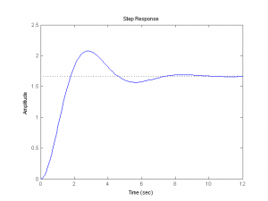
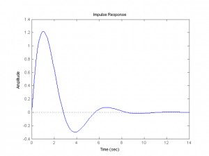
The resulting plots are shown below.
More generally, we can graph the response of an arbitrary linear function u(t) on the time interval [0,T] with the lsim command. Define vector u on a time interval t (in the time domain), and the lsim command graphs the response. Note the similarity between the lsim response and the step response above.
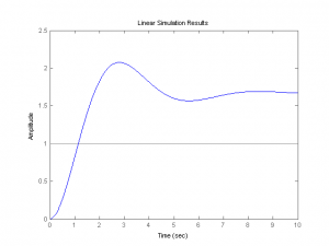
t=linspace(0,10,10000); u=ones(1,length(t));
figure; lsim(tf(B,A),u,t)
We can get the poles and zeros from the transfer function object with the pole() and zero() command. If we are performing multiple operations with the object, it’s worthwhile to create another variable for it.
H=tf(B,A);
pole(H)

ans =

  -1.0000 + 1.4142i
  -1.0000 - 1.4142i

zero(H)

ans =

   Empty matrix: 0-by-1

